
How to transpose data in Excel and Google Sheets
Transposing is turning rows into columns and columns into rows, so a table laid out sideways can be read the normal way. In Excel, copy the range, right-click the target cell and choose Paste Special > Transpose.
By Operelio team · Updated October 8, 2026
On this page10
- 1.Three ways to do it
- 2.How to paste transpose in Excel
- 3.How to transpose with the TRANSPOSE function
- 4.How to transpose columns to rows with Power Query
- 5.How to transpose in Google Sheets
- 6.Transpose or unpivot?
- 7.How to unpivot data in Excel
- 8.Why transpose fails
- 9.Transpose or unpivot a whole file in one step
- 10.Frequently asked questions
Three ways to do it
Paste Special is the quickest. The other two keep a link to the original, so the result changes when it does.
| Method | Use it for | Follows changes to the original |
|---|---|---|
| Paste Special > Transpose | A one-off flip of a range | No, it pastes a fixed copy |
| TRANSPOSE function | A flipped copy that stays up to date in the same workbook | Yes, as you edit |
| Power Query | A report that arrives every week in the same layout | Yes, when you refresh |
How to paste transpose in Excel
Paste Special gives you a fixed copy: change the original later and the transposed copy stays as it was. If you want it to follow the original, use the TRANSPOSE function in the next section.
Copy the range
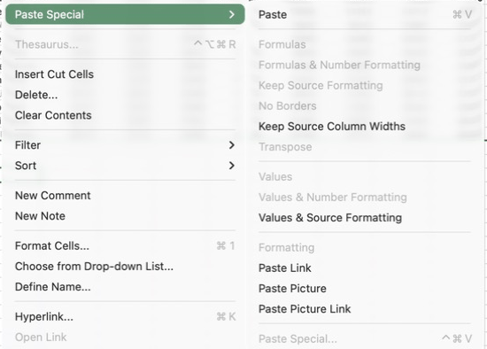
Select the cells to flip, headers included, and press Ctrl+C (Cmd+C on a Mac). Copy, not cut: after a cut, Transpose is grayed out in Paste Special.
Pick a clear spot
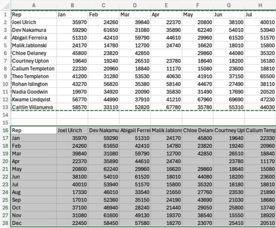
Click the cell where the top left corner of the result should go, outside the range you copied and with enough empty cells to the right and below. A table of 3 rows and 12 columns needs 12 rows and 3 columns.
Paste with Transpose
Right-click the cell and choose Paste Special, check Transpose and click OK. On Windows the keyboard way is Ctrl+Alt+V, then E, then Enter. On a Mac, Ctrl+Cmd+V opens Paste Special, and the right-click Paste Special menu also has Transpose as a one-click option.
Delete the original if you no longer need it
Check the result first, then delete the old rows or columns. Formulas elsewhere in the workbook that pointed at the original cells don't follow the data to its new place (more on that below).
How to transpose with the TRANSPOSE function
=TRANSPOSE(A1:M4) returns the range A1:M4 turned on its side, and stays linked to it: change a value in the original and the transposed copy changes too.
In Microsoft 365 and Excel 2021 or later, type the formula in one cell and the result spills into the cells around it. If any of those cells already hold something, you get a #SPILL! error until you clear them.
In Excel 2019 and earlier, the result has to be entered as an array formula. Select an empty range of the transposed size first (13 rows by 4 columns for A1:M4), type =TRANSPOSE(A1:M4), and press Ctrl+Shift+Enter instead of Enter.
Empty cells in the original come back as 0. To keep them blank, use =TRANSPOSE(IF(A1:M4="", "", A1:M4)).
How to transpose columns to rows with Power Query
Power Query is worth the extra steps when the same report arrives every week: you set the transpose up once and refresh it for each new version.
Load the range into Power Query
Click inside the data and go to Data > From Table/Range. Excel turns the range into a table if it isn't one already, then opens the Power Query Editor. Excel for Mac may not have From Table/Range: save the workbook, then go to Data > Get Data (Power Query) > Excel workbook, pick the file, select the sheet and click Transform data.
Move the headers into the data
Power Query treats the first row as column names, and Transpose would drop them. Go to Home > Use First Row as Headers, open its dropdown, and choose Use Headers as First Row.
Transpose
Go to Transform > Transpose. The rows become columns.
Set the new headers
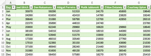
Go to Home > Use First Row as Headers, so the old first column becomes the new header row. The first column keeps the old corner header, such as Rep above a list of months, so double-click it and rename it.
Load it back to Excel
Click Home > Close & Load. The result lands on a new sheet. When the source data changes, go to Data > Refresh All.
How to transpose in Google Sheets
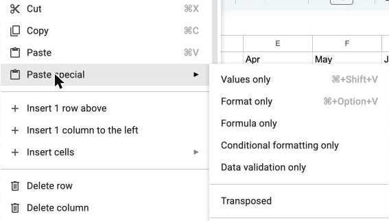
Copy the range, right-click the cell where the result should start, and choose Paste special > Transposed. As in Excel, that pastes a fixed copy.
For a copy that stays linked, type =TRANSPOSE(A1:M4) in an empty cell. The result fills the cells to the right and below on its own, and shows a #REF! error if something is in the way. Unlike Excel, both ways leave empty cells empty rather than turning them into 0.
Transpose or unpivot?
Transpose flips the whole table. Unpivot is turning a wide table into a long one, so each row holds a single record instead of twelve monthly columns. They solve different problems.
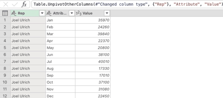
Take a sales report with one row per rep and a column for each month: Rep, Jan, Feb, and so on to Dec. Transposed, the months run down the side and the reps across the top, which is still wide, only in the other direction. Unpivoted, it has three columns, Rep, Month and Sales, with one row for each rep and month: 3 reps across 12 months becomes 36 rows.
Transpose when a table is the wrong way round for reading, such as a report someone built with dates down the side. Unpivot when the data has to go into a pivot table, a chart or a CRM import. A CRM import wants one row per record, which is why a report laid out for a person usually has to be unpivoted first.
How to unpivot data in Excel
Power Query has unpivot built in. Using the sales report above:
Load the table into Power Query
Click inside the data and go to Data > From Table/Range (on a Mac without it, Data > Get Data (Power Query) > Excel workbook, as above).
Select the columns that stay fixed
Click the Rep column header. Ctrl+click any other columns that describe the record rather than hold a value, such as Region.
Unpivot the rest
Go to Transform, click the small arrow beside Unpivot Columns and choose Unpivot Other Columns. Clicking the button itself unpivots the column you selected, the opposite of what you want. The month columns turn into two columns, Attribute (the month) and Value (the sales). Unpivot Other Columns also picks up a month added to the report later, where Unpivot Columns would only take the ones you selected.
Rename and load
Double-click Attribute and rename it Month, and Value to Sales. Then Home > Close & Load.
Without Power Query, Microsoft 365 can unpivot with formulas. With reps in A2:A4, months in B1:M1 and sales in B2:M4, these three formulas, each in its own column, spill the long table: =TOCOL(IF(COLUMN(B2:M4), A2:A4)) for the rep, =TOCOL(IF(ROW(B2:M4), B1:M1)) for the month and =TOCOL(B2:M4) for the sales. An empty sales cell comes out as 0, where Power Query leaves that row out.
Why transpose fails
When Paste Special > Transpose is grayed out, gives an error or pastes something odd, it is usually one of these.
| Problem | What happens | Fix |
|---|---|---|
| The data is an Excel table | Excel's Transpose isn't available for a table. | Convert it first: click inside the table, then Table Design > Convert to Range (the tab is called Table on a Mac). Or use the TRANSPOSE function, which works on tables. |
| You cut instead of copied | After Ctrl+X, Transpose is grayed out in Paste Special. | Copy with Ctrl+C. |
| The paste area overlaps the copied range | Excel won't paste over the cells it is reading from. | Paste somewhere empty, then delete the original. |
| Merged cells | Merged cells don't flip cleanly and can stop the paste. | Select the range and turn off Home > Merge & Center before you copy. |
| Formulas point at the wrong cells | Paste Special copies formulas and shifts their cell references to the new position, which can point them at the wrong data. | Check Values as well as Transpose in Paste Special to paste the results instead of the formulas. |
| Other formulas break | Formulas elsewhere that referred to the original cells still point there, and show #REF! once the original is deleted. | Update them to the new range, or use the TRANSPOSE function and keep the original. |

Transpose or unpivot a whole file in one step
Operelio's Transpose / Unpivot tool reshapes a CSV or Excel file without opening it in a spreadsheet. Upload the file, pick Transpose or Unpivot, and the preview shows the file it will write, with the rows and columns before and after, before you run it.
Transpose flips the whole file and can use its first column as the new header row. Unpivot asks which columns stay fixed and which turn into rows, and what to call the two new columns, such as Month and Sales. A third mode, Group across, does the reverse of unpivot: it turns several rows per company into one row per company with the contacts numbered across, which is the layout some CRM imports want.
All three modes are on every plan, including Free. Your original file is never changed; the result is a new file.
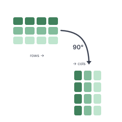
Flip rows and columns, or unpivot wide data into long format, a whole file at a time.
Frequently asked questions
What does transpose mean in Excel?
Turning rows into columns and columns into rows. A table with months across the top and reps down the side becomes one with reps across the top and months down the side. The values don't change, only where they sit.
Where is transpose in Excel?
In Paste Special. Copy the range, right-click the target cell, choose Paste Special and check Transpose. It is also a function, =TRANSPOSE(range), and a button in the Power Query Editor under Transform.
How do I transpose a table in Excel?
Paste Special > Transpose isn't available for an Excel table, so convert it first: click inside the table, then Table Design > Convert to Range, and copy and paste as usual. Or leave it as a table and use =TRANSPOSE, which works on tables.
Does transpose keep formulas?
Paste Special > Transpose copies the formulas and shifts their cell references to the new position, which often leaves them pointing at the wrong cells. To keep the results instead, check both Values and Transpose. The TRANSPOSE function is different: the whole result is one formula linked to the original.
How do I unpivot data in Excel without Power Query?
In Microsoft 365, TOCOL can do it with three formulas: one for the fixed column, one for the old headers and one for the values. In older versions the usual route is copying each month's column under the last by hand. Operelio's Transpose / Unpivot tool does it on the file in one run.
Ready to get started?
Upload a file and run your first transformation. Free, no credit card required.