
How to use VLOOKUP in Excel and Google Sheets
VLOOKUP is the spreadsheet function that pulls a value out of a second table by matching on a shared column. In Excel and Google Sheets the formula is =VLOOKUP(lookup_value, table_array, col_index_num, FALSE).
By Operelio team · Updated October 8, 2026
On this page10
- 1.What is VLOOKUP?
- 2.The VLOOKUP formula, argument by argument
- 3.How to do a VLOOKUP in Excel, step by step
- 4.Before the file goes into your CRM
- 5.How to do a VLOOKUP between two sheets or two workbooks
- 6.How to use VLOOKUP in Google Sheets
- 7.Why is my VLOOKUP not working?
- 8.VLOOKUP vs XLOOKUP
- 9.Match two whole files without a formula
- 10.Frequently asked questions
What is VLOOKUP?
You give VLOOKUP a value to find, such as an email address. It searches the first column of a table for that value, goes across the same row, and returns whatever is in the column you asked for, such as the company name. The V stands for vertical: it searches down a column. Excel and Google Sheets both have it, and the formula is the same in both.
The most common job is joining two exports: a list of leads from one system and a list of accounts from another, matched on email so each lead gets its company, owner or status before the file goes into the CRM.
The VLOOKUP formula, argument by argument
VLOOKUP takes four arguments, in this order:
=VLOOKUP(lookup_value, table_array, col_index_num, FALSE)
| Argument | What it is | Example |
|---|---|---|
| lookup_value | The value to find. Usually a cell on the current row. | A2 |
| table_array | The table to search. VLOOKUP looks for the value in its first column only. | Companies!$A$2:$B$500 |
| col_index_num | Which column of that table to return, counting the table's first column as 1. It counts from the table, not from column A of the sheet. | 2 |
| range_lookup | FALSE finds an exact match. TRUE, or leaving it out, finds an approximate match. | FALSE |
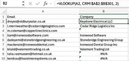
Always end the formula with FALSE unless you are looking up a number in a sorted range, like a tax band. Leave it out and VLOOKUP does an approximate match: on an unsorted list it returns a value from the wrong row, with no error to warn you.
How to do a VLOOKUP in Excel, step by step
The example: a sheet called Leads has email addresses in column A and an empty Company column B. A second sheet in the same workbook, Companies, has Email in column A and Company in column B. The formula fills in each lead's company from the Companies sheet.
Check the lookup column comes first
VLOOKUP only searches the first column of the table you give it, and only returns columns to the right of it. On the Companies sheet, Email is column A, so the table can start there. If the email column sat to the right of Company, you would move it, or use XLOOKUP or INDEX MATCH instead (both are further down).
Start the formula on the first row
On the Leads sheet, click B2 and type =VLOOKUP(A2, so A2, the first lead's email, is the value to find.
Select the table on the other sheet
Click the Companies sheet tab and select A2:B500, or however far your data goes. Excel writes Companies!A2:B500 into the formula. Press F4 (Cmd+T on a Mac) to make it Companies!$A$2:$B$500. The $ signs stop the range from moving down a row each time you copy the formula down.
Finish the formula
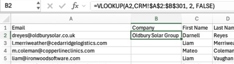
Type , 2, FALSE) and press Enter. The 2 returns the table's second column, Company. Excel takes you back to the Leads sheet, and B2 shows the company for the first email. The whole formula reads =VLOOKUP(A2, Companies!$A$2:$B$500, 2, FALSE).
Copy it down the column
Click B2 and double-click the small square at the bottom right of the cell. Excel copies the formula down as far as the data in column A goes, and each row looks up its own email.
Check the rows that show #N/A
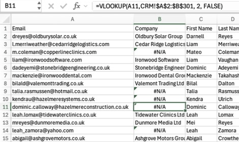
#N/A means that email is not in the Companies sheet's first column. Sometimes that is true. Often it is a stray space or a difference you cannot see, so check a few before you trust them (the fixes are below).
Before the file goes into your CRM
Two things catch people out when the sheet with the VLOOKUP is the file they import.
First, the #N/A cells. Save the sheet as a CSV and each one is written as the text #N/A, which a CRM import reads as a real value. Every contact without a match ends up with #N/A as their company. Wrap the formula in IFNA to leave those cells blank instead: =IFNA(VLOOKUP(A2, Companies!$A$2:$B$500, 2, FALSE), ""). If you change only some cells this way, Excel marks them with a small green triangle because their formula differs from the cells around them. That is a note, not an error.
Second, the formulas themselves. They depend on the Companies sheet, so delete or move it and every cell turns to #REF!. Once the results look right, select the column, copy it, and paste it back with Home, Paste, Paste Values. The companies stay and the formulas go.
How to do a VLOOKUP between two sheets or two workbooks
Between two sheets in the same workbook, the steps above are all there is: the sheet name and an exclamation mark go in front of the range, as in Companies!$A$2:$B$500. Excel adds the name for you when you click across to select. If the sheet name has a space in it, Excel wraps it in single quotes, as in 'Company list'!$A$2:$B$500.
Between two separate workbooks, open both first. Start the formula in the workbook that needs the values, then switch to the other one with View, Switch Windows, and select the range. Excel adds the file name in square brackets and makes the reference absolute on its own: =VLOOKUP(A2, [Companies.xlsx]Sheet1!$A$2:$B$500, 2, FALSE). If the file name has a hyphen or a space, Excel puts single quotes around the file and sheet, as in '[crm-contacts.xlsx]CRM'!$A$2:$B$301. If a CSV copy of the file is open too, Switch Windows lists both, so close the CSV first.
When you close the source workbook, Excel rewrites the reference to include the file's full path and keeps the last values it read. The next time you open the workbook with the formula, Excel warns that it links to external sources and asks you to choose Update or Don't Update. If you move or rename the source file, the link breaks, which is another reason to paste the results as values once they are right.
![Excel's formula bar with a VLOOKUP into another open workbook: =VLOOKUP(A2,'[crm-contacts.xlsx]CRM'!$A$2:$B$301, 2, FALSE).](/guides/vlookup-in-excel/04-other-workbook-formula-crop.png)
How to use VLOOKUP in Google Sheets
The formula is the same. Type =VLOOKUP(A2, Companies!$A$2:$B$500, 2, FALSE) into a Google Sheet with the same two tabs and it returns the same result. Google names the arguments differently (search_key, range, index and is_sorted), but they do the same jobs in the same order.
Google Sheets also assumes a sorted range unless you say otherwise, so it needs the FALSE at the end too. When you press Enter, Sheets usually offers Suggested auto-fill for the rest of the column: click the checkmark to accept it. Otherwise, drag the small square at the bottom right of the cell down the column.
The real difference is looking up from another file. VLOOKUP cannot point at a different spreadsheet directly, so you wrap the range in IMPORTRANGE with the other file's URL, as in the formula below. The first time, the cell shows #REF! until you connect the two files: click the cell and then Allow access. The range names the tab in the other file, so check its name: a spreadsheet made by importing a CSV names its tab after the file.
=VLOOKUP(A2, IMPORTRANGE("https://docs.google.com/spreadsheets/d/...", "Companies!A2:B500"), 2, FALSE)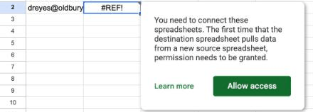
Why is my VLOOKUP not working?
These are the usual causes, with the fix for each.
| What you see | Why | Fix |
|---|---|---|
| #N/A on a value you can see in the table | A stray space before or after the value, in either sheet. Text pasted from web pages can also carry non-breaking spaces, which look the same but are a different character. | Look up the trimmed value with =VLOOKUP(TRIM(A2), ...). If the spaces are in the table, clean that column first with TRIM, plus SUBSTITUTE(A2,UNICHAR(160)," ") for non-breaking spaces. Use UNICHAR, not CHAR: in Excel for Mac, CHAR(160) is a different character. |
| #N/A on IDs, ZIP codes or phone numbers | Numbers stored as text in one sheet and as numbers in the other. 1042 and "1042" never match. | Convert the text column: Excel marks those cells with a green triangle, and the warning menu has Convert to Number. Or match the table's format in the formula, as in =VLOOKUP(A2&"", ...) when the table holds text. |
| #N/A on values that are not in the table | The value is not there. | Wrap the formula in IFNA to show a blank or a word of your choice: =IFNA(VLOOKUP(...), "Not found"). |
| A result from the wrong row, with no error | The fourth argument is TRUE or missing, so VLOOKUP did an approximate match on an unsorted list. | End the formula with FALSE. |
| The wrong column comes back | col_index_num counts from the first column of the table, not from column A. Inserting a column into the table also shifts what the number points at. | Count again from the table's first column, or use XLOOKUP, which does not use a column number. |
| #REF! | col_index_num is larger than the number of columns in the table. | Widen the table to include the column you want, or lower the number. |
| #N/A because the match is to the left | VLOOKUP only searches the table's first column and only returns columns to its right. | Move the lookup column to the front, or use XLOOKUP or INDEX MATCH. |
| Rows further down stop matching | The table range moved when the formula was copied down, because it had no $ signs. | Make the range absolute: $A$2:$B$500. |
VLOOKUP returns the first match it finds. If an email appears twice in the table with two different companies, you get whichever comes first, and nothing tells you there was a second.
VLOOKUP vs XLOOKUP
XLOOKUP is the newer function. It takes the column to search and the column to return as two separate ranges, so there is no column number to count and nothing breaks when a column is inserted. It finds an exact match unless you ask for something else, it can return a column to the left of the one it searches, and it has its own argument for what to show when nothing matches. The worked example becomes =XLOOKUP(A2, Companies!$A$2:$A$500, Companies!$B$2:$B$500, "").
XLOOKUP is in Microsoft 365, Excel 2021 and later, Excel for the web and Google Sheets. It is not in Excel 2016 or Excel 2019, and a file that uses it shows errors when opened there. If anyone who opens the file is on an older version, stay with VLOOKUP.
INDEX MATCH is the older way to get the same flexibility, and it works in every version: =INDEX(Companies!$B$2:$B$500, MATCH(A2, Companies!$A$2:$A$500, 0)). MATCH finds the row number, INDEX returns the value from that row of the column you name, and the 0 asks for an exact match.
Match two whole files without a formula
A VLOOKUP works one cell at a time, and the file has to be clean for it to work. Operelio's Match & pull columns does the same job on two whole files. Upload the file you want filled in and the file the extra columns come from, pick the shared column, and pick which columns to bring across. Every row is matched in one run and you download one combined file.
It also covers what a VLOOKUP cannot. It matches on more than one column at once, such as first name and last name together. Similarity matching catches typos and small differences, like Westmarch Trading in one file and WESTMARCH TRADING LTD in the other. You choose whether to keep every row, only the rows that matched, or every row from both files. The two files can be CSV or Excel, in any mix, and the originals are never changed.
All of it is on every plan, including Free, which reads up to 2,000 rows in each file.

Pull matching columns from a second file on a shared column, without a formula.
Related
Frequently asked questions
What does FALSE mean at the end of a VLOOKUP?
Exact match. FALSE tells VLOOKUP to return a value only when it finds the lookup value itself. TRUE, or leaving the argument out, asks for an approximate match, which assumes the first column is sorted and returns the nearest smaller value. On an unsorted list that is often a value from the wrong row.
Can VLOOKUP look to the left?
No. It only searches the first column of the table and only returns columns to the right of it. To return a column on the left, move the lookup column to the front, or use XLOOKUP or INDEX MATCH, which take the search column and the return column separately.
Can VLOOKUP return more than one column?
One formula returns one column, so the usual way is to copy it across and change the column number in each copy. In Microsoft 365 and Excel 2021 or later, a list of column numbers returns several at once: =VLOOKUP(A2, Companies!$A$2:$D$500, {2,3,4}, FALSE) fills three cells to the right. In Google Sheets, wrap that in ARRAYFORMULA. Without it, Sheets returns only the first of the columns, with no error.
Ready to get started?
Upload a file and run your first transformation. Free, no credit card required.